# Author:       Ariel Aguilar Gonzalez
# Date:         Saturday, July 16 2016
# Tile:         Are Injuries Really An Excuse?
# Description:  Using Historical EPL Data to Examine the Effect of Injuries
#  ----------------------------------------------------------------------------

#-------------------------------------------#
#         Load Data and Libraries           #
#-------------------------------------------#

library(ggplot2)
library(ggrepel)
library(car)
library(scatterplot3d)
library(stargazer)

# Import Dataset with Injury, EPL Performance Data
# Sources: Premier League, Football Data, Physio Room, Wikipedia
Regression_Data <- read.csv("...Regression_Data.csv")

# Attach the variable names to be able to call variables
attach(Regression_Data)

#-------------------------------------------#
#          Basic Data Exploration           #
#-------------------------------------------#

# Basic Summary Stats
mean(Days.Lost.to.Injury)
# 1001 days!
mean(Number.of.Injuries)
# 26 injuries!

# Look at different correlations to help determine independent variables in regression
cor(Pts, Tackles)
cor(Pts, Interceptions)
# Tackles have a stronger correlation with Points
cor(Pts, Red.Cards)
cor(Pts, Booking.Points)
# Booking Points have a stronger negative correlation with Points
cor(Pts, Number.of.Injuries)
cor(Pts, Days.Lost.to.Injury)
# Days Lost to Injury have an actual negative correlation with Points

# Create correlation plot for Points and Injuries
cor.vec <- round(cor(Pts, Days.Lost.to.Injury),2)
txt<-paste("Correlation is", cor.vec)
sources <- "Data Sources: Premier League Stats Centre\n Football Data.co.uk\n Physio Room"

inj.pts <- ggplot(Regression_Data, aes(x=Days.Lost.to.Injury,y=Pts))
inj.pts + geom_point()+theme(legend.position="none")+ylab("Points")+
  xlab("Number of Days Lost to Injury") + geom_smooth(linetype="dashed", method="lm")+
  theme(axis.title.y = element_text(angle = 90), plot.title = element_text(face="bold"))+
  ggtitle("Injuries and Points Don't Seem To Be Related?!")+
  annotate("text", x = 1900, y = 17, label = txt, fontface="bold",size=4) +
  annotate("text", x = 1900, y = 10, label = sources, fontface="bold",size=2.5)
dev.copy(jpeg, 'injurycorr.jpeg')
dev.off()

# Let's make a histogram plot of injuries

inj <- ggplot(data=Regression_Data, aes(Regression_Data$Days.Lost.to.Injury)) + geom_histogram(aes(y=..density..))
inj + geom_density(col=2) +
  labs(title="Histogram for Injuries") + labs(x="Days Lost to Injuries", y="Count")
dev.copy(jpeg, 'injuryhist.jpeg')
dev.off()

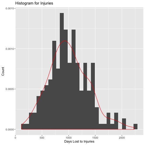
# Look like they're normally distributed, especially given the small sample
# Not important for OLS Regression but good to know, espcially for student's t test later

#-------------------------------------------#
#         Regression Modelling              #
#-------------------------------------------#

## OLS Regression

# Define the model using variable names
y <- Pts
x1 <- Shots
x2 <- Touches
x3 <- Tackles
x4 <- Booking.Points
x5 <- Days.Lost.to.Injury

model.1 <- y ~ x1 + x2 + x3 + x4 + x5
model.2 <- y ~ x1 + x2 + x4
model.3 <- y ~ x1 + x2 + x4 + x5 + I(x1^2) + I(x2^2) + I(x4^2) + I(x5^2)
model.4 <- y ~ x1 + x2 + x4 + x5 + I(x4^2) + I(x5^2)
model.5 <- y ~ x1 + x2 + x5 + I(x5^2)
model.6 <- y ~ x1 + x2 + x3 + x5 + I(x5^2)
model.7 <- y ~ x1 + x2 + x4 + x5 + I(x5^2)
model.8 <- y ~ x1 + x2

# Estimate the model and store the results
reg.model.1 <- lm(formula= model.1, data= Regression_Data)

# Regression results
# Will evaluate the models by adjusted R squared value

summary(reg.model.1)
# Shots and Touches come up as significant
# Adjusted R squared value of 59.3%

reg.model.2 <- lm(formula= model.2, data= Regression_Data)
summary(reg.model.2)
# Again Shots and Touches come up as significant, but not booking points
# Adj R squared of 58.8%

reg.model.3 <- lm(formula= model.3, data= Regression_Data)
summary(reg.model.3)
# Here Shots, Touches and Days Lost to Injury come up as significant
# Adj R squared of 62.2%

reg.model.4 <- lm(formula= model.4, data= Regression_Data)
summary(reg.model.4)
# Shots, Touches and Injuries significant
# Adj R squared of 59.9%

reg.model.5 <- lm(formula= model.5, data= Regression_Data)
summary(reg.model.5)
# Everything significant, Adj R squared of 59.7%

reg.model.6 <- lm(formula= model.6, data= Regression_Data)
summary(reg.model.6)
# Tackles are not significant, Adj R squared of 59.8%

reg.model.7 <- lm(formula= model.7, data= Regression_Data)
summary(reg.model.7)
# Booking points not significant, adj R squared of 59.7%

# Two final candidate models, model 3 and 4

# Export the model summaries
stargazer(reg.model.3,reg.model.4,type="html",dep.var.labels = "Points",
          covariate.labels=c("Shots","Touches","Booking Points","Days Lost to Injury","Shots (squared)","Touches (squared)",
                             "Booking Points (squared)", "Days Lost to Injury (squared)"), out="final.htm")

#-------------------------------------------#
#            Evaluate Models                #
#-------------------------------------------#

# Create train and test splits of the data
n_train <- round((nrow(Regression_Data)*2)/3,0)
set.seed(1986)
train_index <- sample(1:nrow(Regression_Data), n_train)

X_train <- Regression_Data[train_index,]
X_test <- Regression_Data[-train_index,]

# Train models
model.3.train <- lm(Pts ~ Shots + I(Shots^2) + Touches + I(Touches^2) + Booking.Points
                    + I(Booking.Points^2) + Days.Lost.to.Injury + I(Days.Lost.to.Injury^2), 
                    data= X_train)
model.4.train <- lm(formula= Pts ~ Shots + Touches + Booking.Points
                    + I(Booking.Points^2) + Days.Lost.to.Injury + I(Days.Lost.to.Injury^2), 
                    data= X_train)

benchmark.train <- lm(formula= Pts ~ Shots + Touches,data= X_train)

# Create predictions
model.3.preds <- round(predict(model.3.train, X_test))
model.4.preds <- round(predict(model.4.train, X_test))
benchmark.preds <- round(predict(benchmark.train, X_test))

# Measure accuracy (mean absolute error)

model.3.mae <- mean(abs((X_test$Pts - model.3.preds)))
# 9.64
model.4.mae <- mean(abs((X_test$Pts - model.4.preds)))
# 9.81
benchmark.mae <- mean(abs((X_test$Pts - benchmark.preds)))
# 9.76

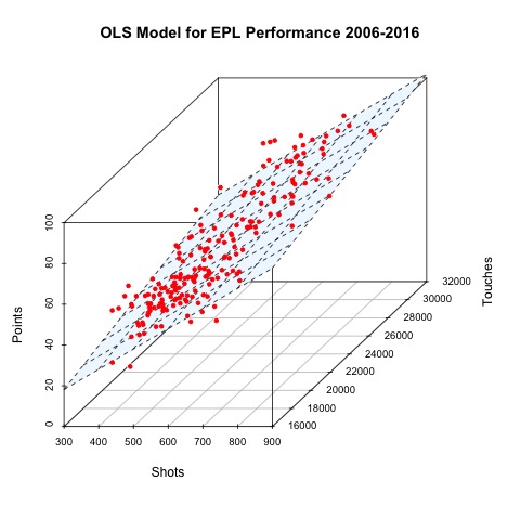
# Just for fun, make 3D Plot of model 8, linear regression model
reg.model.8 <- lm(formula= model.8, data= Regression_Data)
s3d <- scatterplot3d(x=x1,y=x2,z=y,color="white", main="OLS Model for EPL Performance 2006-2016", xlab="Shots", ylab="Touches", zlab="Points")
s3d$plane3d(reg.model.8, draw_polygon = TRUE, polygon_args=list(border=NA, col="aliceblue"))
s3d$points3d(x=x1,y=x2,z=y,col="red", pch=20)
# SO COOL!!
dev.copy(jpeg, 'regvis.jpeg')
dev.off()

#-------------------------------------------#
#            Analysis by Group              #
#-------------------------------------------#

# Import data frame of solely UCL, Relegated, and Middle of the Pack
UCL <- read.csv("...UCL.csv")
Relegated <- read.csv("...Relegated.csv")
Middle <- read.csv("...Middle.csv")
# UCL contains 40 observations
# Relegated contains 30 observations
# Middle contains 130 observations
# All are too small to complete regression analysis

# Plot scatterplot, calculate mean, correlation of new data frames

# Average Injuries within the groups
mean(Regression_Data$Days.Lost.to.Injury)
# 1001.3
mean(Relegated$Days.Lost.to.Injury)
# 1042.7
mean(UCL$Days.Lost.to.Injury)
# 1038.2
mean(Middle$Days.Lost.to.Injury)
# 980.3

# Correlation of Points to Injuries within the groups
cor(Regression_Data$Pts, Regression_Data$Days.Lost.to.Injury)
# -0.0178
cor(UCL$Pts, UCL$Days.Lost.to.Injury)
# -0.2105
cor(Relegated$Pts, Relegated$Days.Lost.to.Injury)
# 0.0006
cor(Middle$Pts, Middle$Days.Lost.to.Injury)
# -0.0066

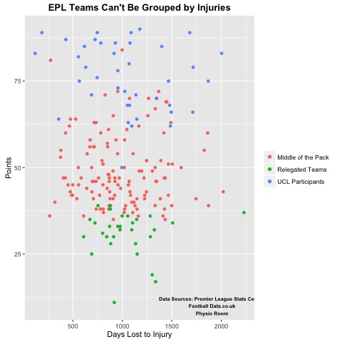
# Appears that Injuries are more costly to elite teams
# But not enough data to verify with regression analysis
# Would need either more seasons or match data

# Two Sample t tests

t.test(Regression_Data$Days.Lost.to.Injury, UCL$Days.Lost.to.Injury)
# Null is that means are equal
# P value is 0.625, fail to reject null

t.test(Regression_Data$Days.Lost.to.Injury, Relegated$Days.Lost.to.Injury)
# Same null as previous test
# P value is 0.518, fail to reject null

t.test(Regression_Data$Days.Lost.to.Injury, Middle$Days.Lost.to.Injury)
# P value is 0.614, fail to reject null

# It appears that Elite,Bad and Middle teams do not suffer more injuries than the population
# Rather injuries seem to be more costly to Elite teams, though just as numerous

# Scatterplot

Injury_Groups <- ggplot(Regression_Data, aes(x=Days.Lost.to.Injury, y=Pts)) +
  geom_point(data = Middle, aes(x=Days.Lost.to.Injury, y=Pts, colour="Middle of the Pack")) +
  geom_point(data=UCL, aes(x=Days.Lost.to.Injury, y=Pts, colour="UCL Participants")) +
  geom_point(data = Relegated, aes(x=Days.Lost.to.Injury, y=Pts, colour="Relegated Teams")) +
  theme(axis.title.y = element_text(), plot.title = element_text(face="bold"))+
  ggtitle("EPL Teams Can't Be Grouped by Injuries") + labs(x="Days Lost to Injury", y="Points") +
  theme(legend.title=element_blank()) + annotate("text", x = 1900, y = 10, label = sources, fontface="bold",size=2.5)
Injury_Groups
dev.copy(jpeg, 'injurygroups.jpeg')
dev.off()